Most people use maps on a regular basis for a variety of purposes. Those of us interested in river systems typically rely on this aerial, two-dimensional perspective in a professional or recreational context. While maps represent extremely useful tools to locate streams, lakes and glaciers, they lack information about the third dimension: elevation. Hydrodynamic models (see example of the Klondike River), developed through the processing of high-accuracy spatial and elevation data, are commonly used by hydrology engineers over relatively short river distances, but for long river distances, the profile of rivers remains largely unknown.
Figure 1 presents the longitudinal profile of a river system, in this case, the Yukon River in Yukon. Instead of showing the Yukon River and its main tributaries from above, it brings them together on the same vertical plane, as if they were flowing next to each other. In other words, it expresses the elevation of their water surface (above sea level) as a function of the distance from a common point (in this case, the Alaska Border).

Figure 1. Side view (elevation expressed as a function of distance) of the Yukon River system, including major tributaries.
How was this produced?
Our summer student, Joe Boyd, under the supervision of Stephanie Saal, Research Professional and GIS expert, used the Arctic Digital Elevation Model to extract elevation data at every 100 m along several rivers of the territory. Elevation errors were corrected using a custom algorithm. The approximate thalweg (line where the flow is usually the fastest) was manually digitized based on the Arctic DEM and satellite imagery. Therefore, the profile of each river may correspond (in the case of steep, linear channels), or not (in the case of low-gradient, meandering channels), to the slope of the valley that the rivers have carved over time.
What does this type of graph reveal?
Several assessments can be performed using the data presented in Figure 1. For example, despite them flowing in largely different valleys, the Yukon River, the lower Stewart River, the lower Pelly River, and the Teslin River are characterized by virtually identical slopes (about 0.05% or 0.5 m per km of river). Just through field observations, it appears obvious that the Klondike River is steeper than the Yukon River near Dawson; however, the data helps specify that it is actually 5 times steeper (the water surface elevation loss going downstream on the Klondike River is about 2.5 m per km). Also of interest is that upstream of the community of Ross River, the upper Pelly River is steeper (it gains elevation over a shorter distance) than the Ross River. Llewellyn Glacier, the melt waters of which flow into Atlin Lake and then into the Yukon River, loses (or gains, going upslope) as much elevation over 11 km as the Yukon River over 1100 km.
How is this data useful to practitioners?
The gradient of a river influences important hydrological factors such as the response time of a watershed (how fast the river system reacts to weather forcing). For example, during intense snowmelt or rain events, it is expected that the Pelly River would respond faster than the Ross River. River ice processes are also directly linked to the gradient of specific river segments: in steep river sections, the ice cover will tend to form later in the fall (because the water flows too fast to freeze) and to breakup first in the spring (because the drag force acting on the ice cover is higher).
Other advantages of developing this type of tool include:
- Supporting the design of hydraulic structures, the development of land parcels located on the floodplain, and the preparation of flood maps.
- Contributing to the development of more reliable hydrological models and breakup forecast models (for flood forecasting).
- Tracking the impact of climate change and human activity on the stability and alignment of river channels in alluvial plains.
- Providing information to long distance paddlers about the location of steeper (potentially faster or slower, in the case of white water) and flatter river sections.
Practical example
As some readers may know, the community of Fort McPherson, located on the banks of the Peel River some 45 km upstream of the Mackenzie River in the Northwest Territories, was significantly affected by an ice jam during the spring of 2023. Could this event have been predicted several hours or even days in advance?
During the following summer, Adam Scheck, pilot at Alkan Air, reported major damage to floodplain vegetation near the Snake River confluence with the Peel River (Km 275), and wisely attributed this to dynamic ice processes (ice jam formation and release events). The extent of the damage was quite impressive, with trees flatten down at several locations, including at one location where the ice run plowed through over 800 m of mature forest (Sentinel-2 images presented in Figure 2).
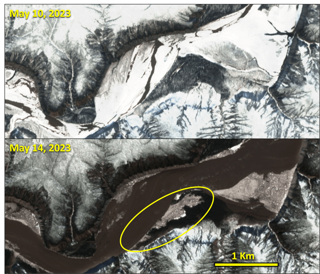
Figure 2. Satellite image showing Km 285 (upstream of the Mackenzie River) of the Peel River on May 10 (above, partially degraded ice cover) and May 14 (ice jam mobilized downstream with damage vegetation near the center of the image.
The preliminary analysis of low-accuracy elevation data suggests that the ice jam formed in a very low gradient reach of the Peel River near Km 285 (upstream of the Peel confluence with the delta of the Mackenzie River), as presented in Figure 3. This is not surprising as a reduction in channel slope is often associated with the formation of ice jams (the ice run coming from upstream loses energy and momentum at such locations). Upon release, these ice jams can break an intact ice cover over several tens of river kilometers to form larger ice jams further downstream.
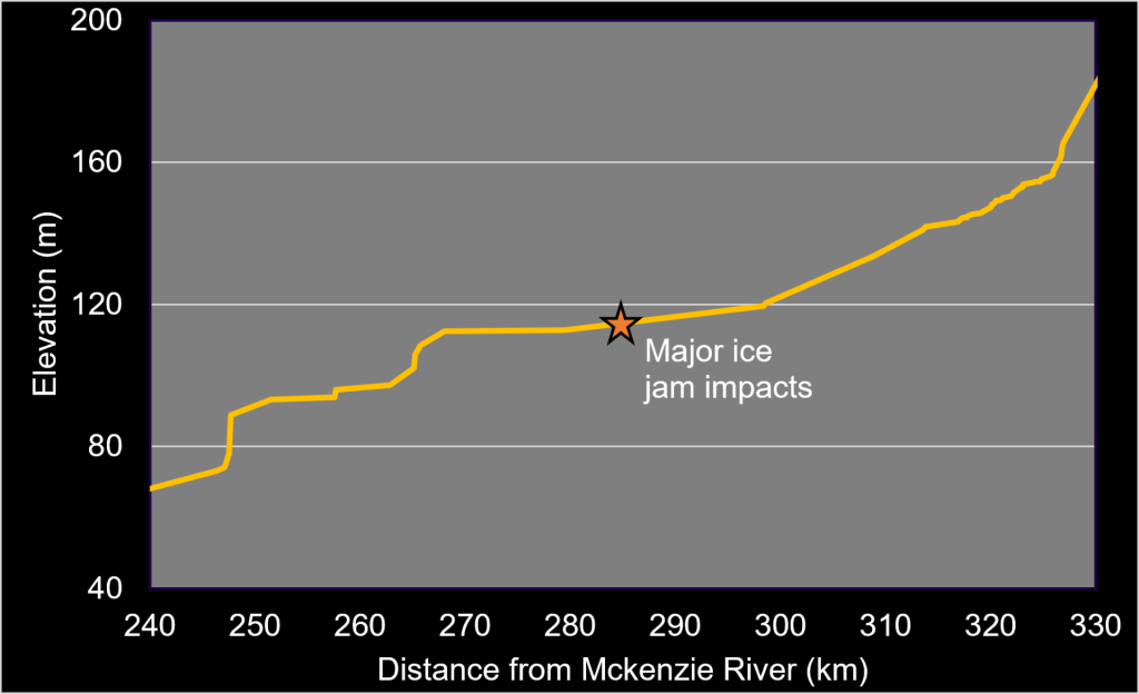
Figure 3. Approximate profile of the Peel River between Km 240 and 330 (above the delta of the Mackenzie River) showing the location of major ice damage to vegetation.
On May 14, 2023, a long ice run was moving down the Peel River towards Fort McPherson. The Water Survey of Canada station, located upstream of the community, was damaged by ice slabs pushed against the bank, and the community was flooded by an ice jam.
Further analyses of the Peel River profile and alignment, together with an investigation of historical satellite images, may help confirm if the formation of a major ice jam near the Snake River confluence correlates with ice jam damage near Fort McPherson in the following hours or days.
Future Steps
The ambition of our research team is to continue working on four aspects of this project:
- Elevation accuracy: The data extracted from the Arctic DEM remains highly inaccurate at a fine scale and may contain large gaps, especially over large (wide) rivers. For example, the White River data presented in Figure 1 shows a vertical step that is not real nor realistic. Our goal is to use high resolution elevation data from a satellite mission that was recently launched: SWOT (Surface Water and Ocean Topography, from NASA).
- Coverage expansion: All major rivers of Yukon will be processed, including in the Liard and Alsek River basins. As interest arises, smaller tributaries could be added to the project.
- Traditional names: Rivers and streams in Yukon had names well before western explorers and stampeders arrived. Previous blog posts attempted to respectfully include Traditional names for rivers and lakes. Since some Traditional names were uncertain when preparing this blog post, in a perspective of consistency and equality, it was decided to adopt western names. However, as one of many steps towards reconciling worldviews, our team will continue collaborating with First Nations with the aspiration of adopting Traditional names.
- Visualization tool: Our team hopes to create a website that will allow users to select and compare the profile and elevation of specific rivers and river segments in a two-dimensional or three-dimensional environment.
If readers are interested in this project, our team would like to hear their comments and discuss potential pilot projects and partnerships.