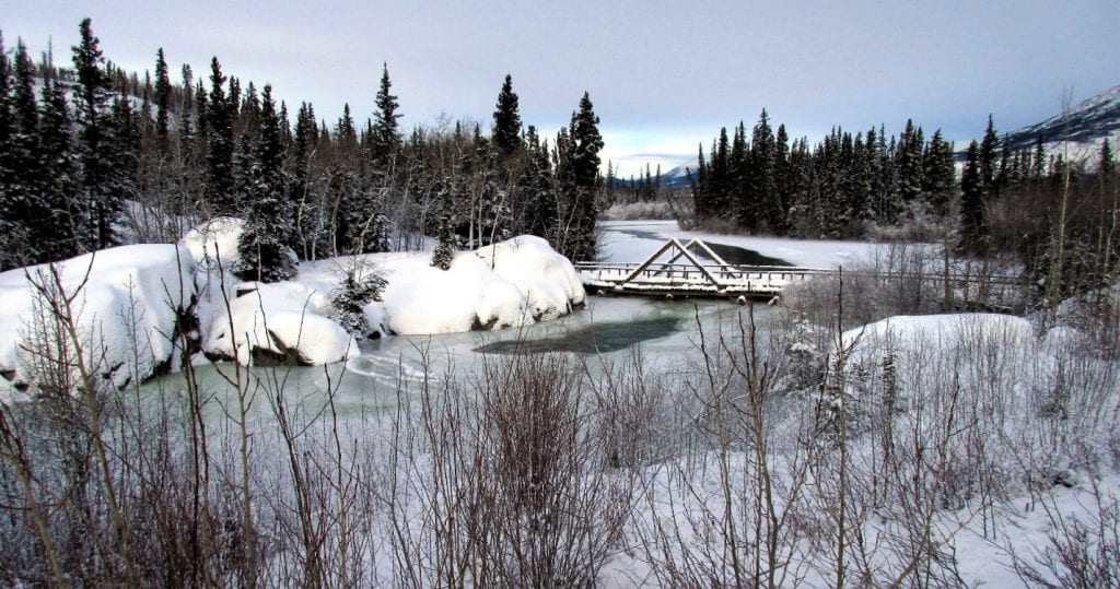
Satellite radar imagery is commonly used to detect ice on large rivers in the context of river ice formation, ice jam flood forecasting, flow management, and navigation. Products from the Sentinel-1 satellite come in 10m x 10m resolution (or coarser) and have been used to classify ice on rivers wider than 100m. However, this resolution presents challenges for detecting ice on narrow rivers. In this study, we examine the feasibility of detecting the commonly used channel surface classes (e.g., open water, sheet and rubble ice) on a narrow, 15m to 50m wide river, by examining Sentinel-1 imagery of the Äshèyi Chù (Aishihik River, Figure 1) on the Traditional Territory of the Champagne and Aishihik First Nations, in the Yukon. These findings were presented at the 22nd Workshop on the Hydraulics of Ice-Covered Rivers.
Context
This study was conducted in the context of the “The Äshèyi Chu/ Aishihik River – River Ice Model” project. The project is a collaboration between Champagne and Aishihik First Nations, Yukon Energy Corporation, Morrison Hershfield (consultant), Government of Yukon, Yukon University, and the University of Alberta.
The project aims to develop a numerical river ice model to simulate winter ice processes and water levels on the Äshèyi Chu downstream from Aishihik Generating Station. The model is intended to inform strategic flow management to reduce the occurrence of overbank icing and winter flooding that impacts the Äshèyi Chu floodplain.
To build the river ice model, an understanding of common ice-bridging locations (river segments where the ice cover extends from bank to bank) is required. Winter conditions on the river are monitored using game cameras and Unmanned Aerial Vehicle (UAV) surveys. However, adding information on the first ice bridging locations based on Sentinel-1 imagery helps to expand our knowledge of river ice formation through time and space.
How does radar “see” ice?
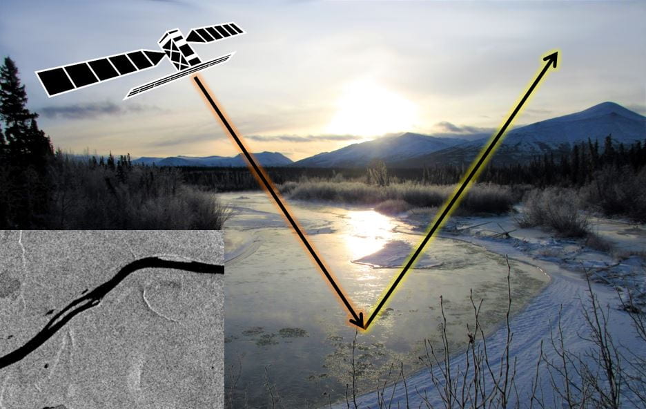
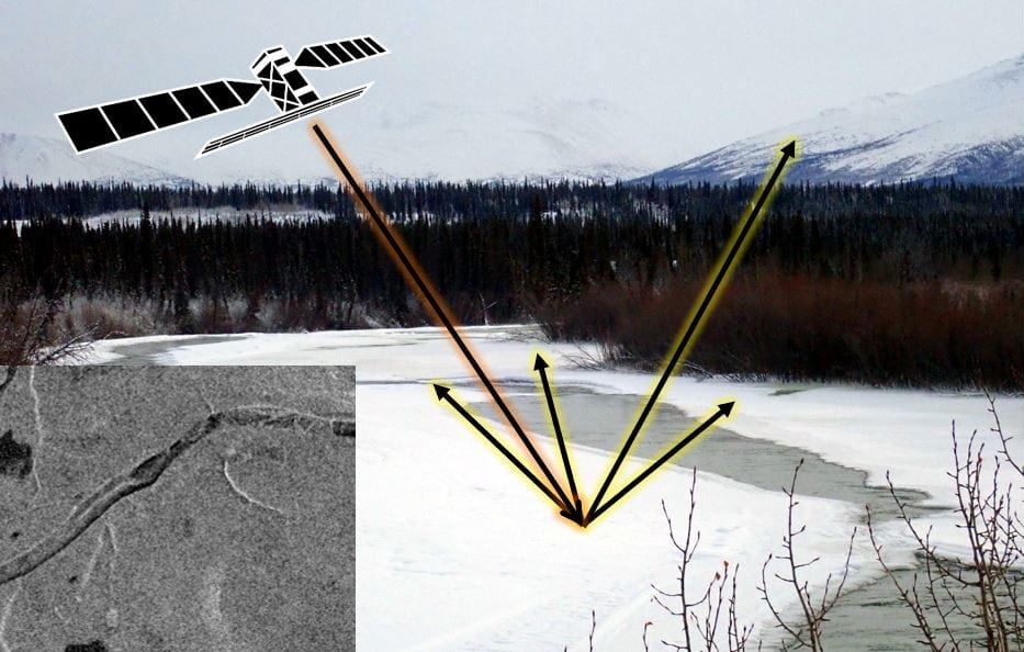
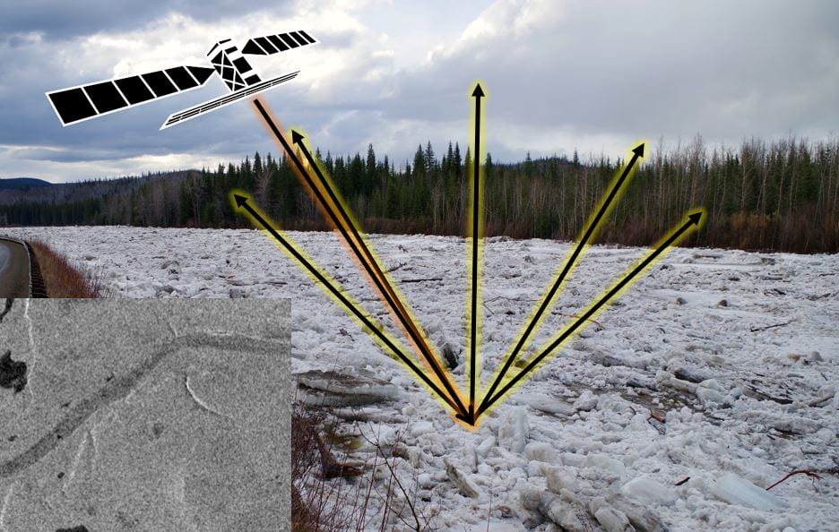
A Synthetic Aperture Radar (SAR) satellite “sees” the landscape differently than we do. Our eyes, as well as a regular handheld camera, receive the amounts of red, green, and blue sunlight reflected by an object. Radar, on the other hand, gathers information about the roughness of a surface. The satellite sends out a signal that will interact with the structure of a surface. Water is a specular surface that will reflect all the sent-out waves away from the satellite (Figure 2). Since the satellite does not receive a return signal, the area will appear dark. Sheet ice has some roughness, resulting in some of the signal being scattered back to the satellite (Figure 3). Rubble ice is rougher than sheet ice or water and the radar signal will interact much more with this uneven terrain; therefore, a higher amount of the signal is scattered back to the satellite, and the area will show up bright (Figure 4).
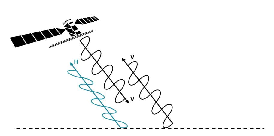
While other imaging satellites commonly look straight down, Sentinel-1 is side looking and looks at the earth on an incidence angle between 29.1° – 46.0°. Radar satellites may send and receive waves in two different polarizations: vertical and horizontal. Polarization refers to the orientation of the radar waves (see Figure 5). At 10m resolution, the Sentinel-1 satellite sends a signal in vertical polarization and can receive it in both vertical and horizontal polarization. Objects such as vegetation canopy cause the signal to bounce around several times before being sent back to the satellite. This has a depolarizing effect and sends a horizontal wave back.
Classification
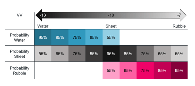
Three ortho mosaics (photogrammetrically orthorectified mosaics created from an image collection) from UAV flights were collected within one day of Sentinel-1 imagery (when ice cover was not quickly changing, as confirmed by automated cameras). Among the ortho mosaics, areas known to represent water, sheet ice, and rubble ice were selected and used to derive a distribution of vertical-vertical polarization (VV) and vertical-horizontal polarization (VH) metrics for each class using corresponding Sentinel-1 datasets. Since the separation between classes was not satisfying for VH polarization, only VV polarization was used for classification. Values were converted into probabilities for the given classes. Figure 6 illustrates the classification scheme. River sections near steep slopes, such as long stretches of cut banks parallel to the river, were removed from the classification to avoid potential false interpretations. Due to the side-looking nature of the satellite, a steep slope facing away from the satellite is invisible to the sensor and would look very dark (similar to water) whereas one facing towards the satellite would appear very bright (like an ice jam or even brighter, as would be the case with a flooded forest).
Salt and pepper
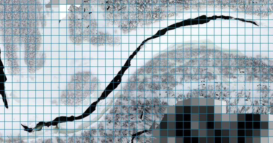
Radar imagery has a typical “salt and pepper” look to it. This noise, called “speckle”, is due to multiple features of varying roughness interacting with the radar signal within one pixel, as well as structures within the same surface type being hit by the radar waves at different angles. Commonly, images are averaged either over multiple images or over multiple grid cells to reduce this noise and create a smoother image. In this specific case, for a narrow river, we cannot afford either of these filtering methods. This is because the river coverage changes too quickly to be filtered over multiple images of different time stamps. Moreover, the river is too narrow to apply a spatial filter over several grid cells. Instead, speckle (Figure 7) was addressed by calculating a minimum significant classification area size and assuming smaller clusters as speckle. Based on summer (ice-free) images of the river, speckle produced clustered features that were 12 pixels or less. We, therefore, consider 12 pixels (i.e. 1200m2) as our minimum threshold for classifying water, sheet and rubble ice units from this dataset.
Outcomes
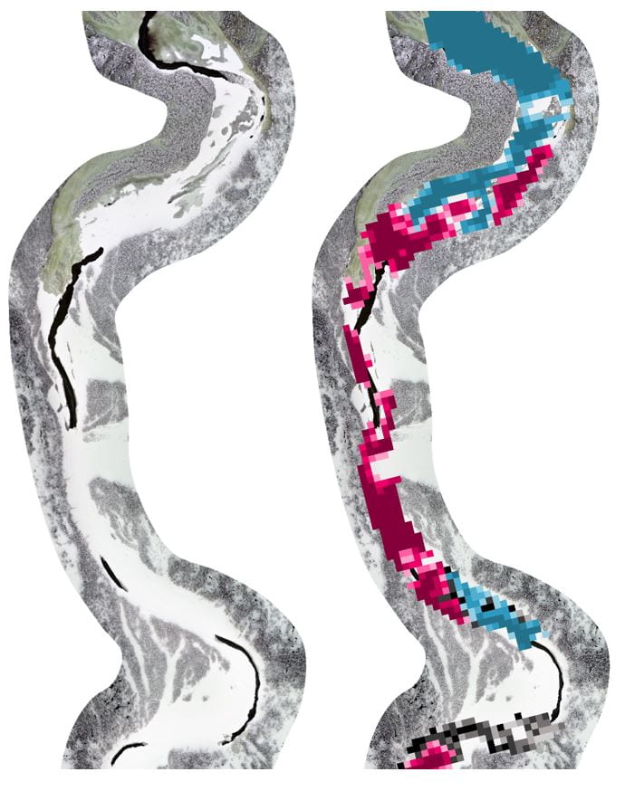
The algorithm was applied to the three available UAV winter ortho mosaics. Figures 8 and 9 show two sections of UAV ortho mosaics (left) and the classification based on Sentinel-1 radar imagery (right).
An upper section of the river (5km below the tailrace), presented in Figure 8, shows a several hundred meters long ice jam and snow-covered rubble ice that was detected in the SAR image (coloured in magenta on the right). We can also see a section of flooded ice and some open water (coloured in teal on the right). In the case of flooded ice, the radar signal interacts with the water on top of the ice instead of the ice underneath, and the satellite only observes water. A potential solution to help differentiate between open water and flooded ice would be to develop a logic-driven algorithm that considers a section’s surface channel classification before and after the image in question. Future research is planned to develop and evaluate the capabilities of this technique.
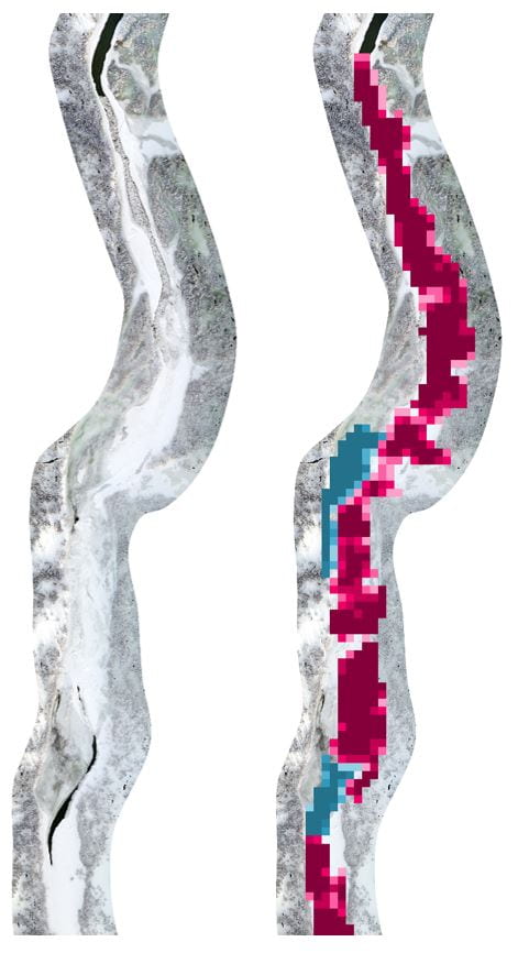
Figure 8 shows a combination of open water and flooded border ice in another upper section of the river (11km below the tailrace). We can see that some ice-covered sections were falsely classified as water. This false classification may be due to wet snow, which interacts with the radar signal similarly to water. The bottom section shows some correctly identified sheet ice (coloured in grey). Border ice with narrow open water was observed to be classified as either of the three classes or removed as speckle. However, the width of the classified band was usually narrower, and we may be able to add a fourth class, “border ice with narrow open water”, by considering the shape of the classified area (object-based classification). Again, future research will show the potential of this approach.
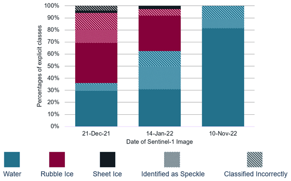
Compiled results indicate that 73% of channel surface pixels are classified correctly, 14% incorrectly, and 13% removed as speckle (Figure 10). Sheet ice, which is structurally in the transition zone between water and rubble ice, had the least identification success.
Conclusion
Classifying ice cover types based on radar satellite products in narrow rivers is possible. While separating sheet and rubble ice can be challenging, distinguishing between ice cover and water was very successful, which is the primary use of this study in its larger context. The classification can be refined using object-based methods as well as a logic-driven approach.